What is Cp and Cpk
Basically, for a process Cp and Cpk are taken as short-term prospective capability measures. In Six Sigma it is desired to define quality of the processes in terms of sigma. The rationale behind this is that it offers a stress-free manner to state the capability of different processes for which a common mathematical framework is used. So, in a nutshell Cp and Cpk are utilized for Process Capability.
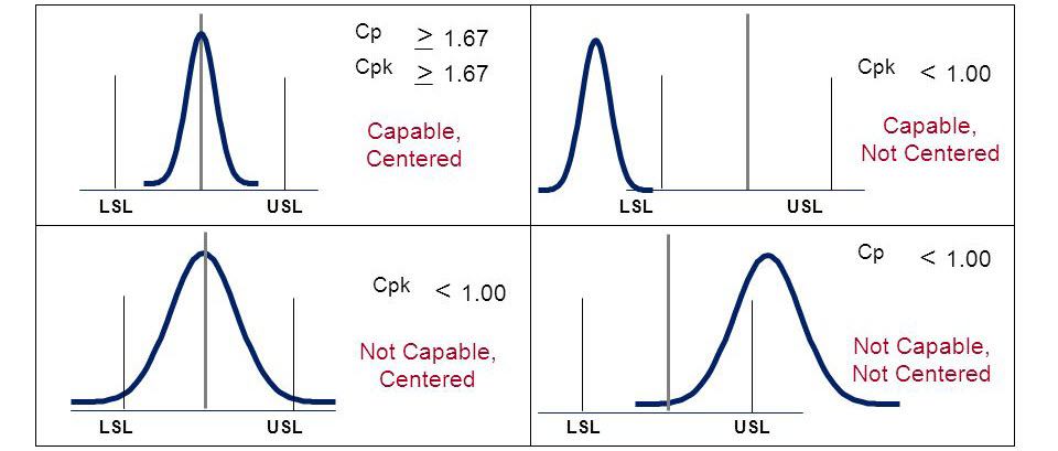
Cpk is an index (a simple number) which measures how close a process is running to its specification limits, relative to the natural variability of the process. The larger the index, the less likely it is that any item will be outside the specification.” Usually Cp & Cpk are used once a process has got steadiness or statistical control. This occurs frequently with a mature procedure being around for a time. The process sigma value defined from the moving range, range or Sigma control charts is used for the process capability. The ‘k’ represents ‘centralizing factor.’ The index considers the fact and possibility of our data not being centered. Cp and Cpk calculates the consistency of our proximate average performance.
Furthermore, Cp and Cpk can be beneficial to a great extent for identifying that the process has got the capability of producing products or services which fit within the required specification. If you hunt our shoot targets with bow, darts, or gun try this analogy. If your shots are falling in the same spot forming a good group this is a high Cp, and when the sighting is adjusted so this tight group of shots is landing on the bullseye, you now have a high Cpk.”
Cp should always be greater than 2.0 for a good process which is under statistical control. For a good process under statistical control, Cpk should be greater than 1.5. Lets look at how to calculate Cp and Cpk.
How to Calculate Cp and Cpk
Let us consider an example which facts the effect that the different methods of how to calculate Cp and Cpk can have over the outcomes of a study process. An organization creates a product that’s satisfactory measurements, formerly identified by the customer, range from 155 mm to 157 mm. The first 10 parts were gathered as samples during a period of 28 days manufactured by a machine that makes the product and operates just during one period.
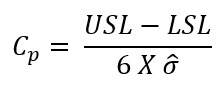
From the formula given below we can calculate the Cp rate of capability:
Here ‘s’ stands for the standard deviation for a population derived from:

Here s-bar standing for the mean of deviation for each rational subgroup and c4 stands for a statistical coefficient of correction. In the given case, the formula takes into account the quantity of variation given by standard deviation and a suitable gap acceptable by specified limits regardless of the mean. The outcomes reveal the population’s standard deviation, assessed from the mean of the standard deviations within the subgroups as 0.413258, which creates a Cp of 0.81.
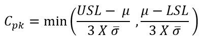
While defining the concept of control graphics a concept of a rational subgroup was developed by Shewart. It includes a sample in which the data differences within a subgroup are reduced and on the other hand the dissimilarities between groups are increased. It gives us the opportunity of having a perfect identification of the ways in which the process parameters transform along a time continuum. In the above mentioned example, the applied process in order to gather the samples permits responsiveness of all daily collections as a specific rational subgroup. From the formula given below we can calculate the Cpk capability rate:
For standard deviation we will consider the same criteria. In addition to the variation in quantity for the given case, the process mean has an impact on the indicators as well. For the reason that the process is not centralized in a perfect way, the mean is near to one of the limits and, consequently, shows a greater chance of not attaining the targets of process capability. In the above mentioned example, specification limits are stated as 155 mm and 157 mm. The mean (155.74) is nearer to one of them as compared to the other, indicating a Cpk factor (0.60) that is below the Cp value (0.81). This point towards that the LSL ((Lower Specification Limit) is more challenging to reach as compared to the USL (Upper Specification Limit). More to the point, non-conformities occur at both ends of the histogram.


